Data Scraping and Model Training
Contents
- Model Description
- Scraping website for Data
- Generating Features
- Retreatment of data
- Model Fitting
- Saving the Model for Evaluation and Predictions
exec(open("Function.py").read())
%matplotlib inline
Model Description
To generate the model and keep the code organized, we have created a class NBAWinProbability(), that takes on arguments for the whether to include the team statistics in the model, the seasons of interest and the folder for where to keep the data. To begin using the model we must call the instance and pass along the arguments as seen below. We can also use the default arguments that are included in the function. Here instead of considering all seasons from 2013 to 2018, we consider only this year’s season for ilustration.
Model=NBAWinProbability(Seasons=[2018])
Scraping website for Data
To scrape for the data, we use the built in function ScrapeData(). This will go to the seasons requested above and will generate data in the Data folder for each game. It will also create a list of .csv, each of them will contain the play-by-play data of a certain game. Also, don’t worry about running it twice. The function is smart enough to recognize that files in the folder exist. So if for some reason the internet connection is dropped, just run it again and it will pick up where it left off.
Model.ScrapeData()
    Creating Data CSV 100.0% Completed
Scrape Data Completed!
The generated list of files look like following:
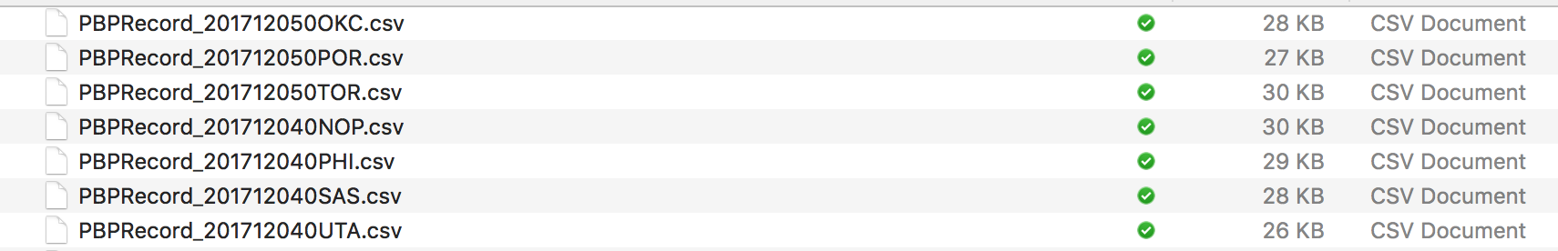
Inside each .csv file there is in detailed play by play data,
Generating Features
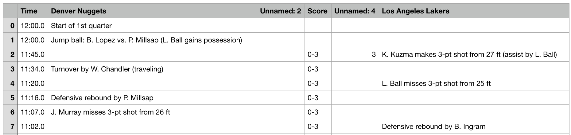
With the list of play by play data, we need to transform them into features that can be trained by ML models. From the data sheet we can extract four types of important information: the time remaining, the name of two teams, their scores and events in string. In events, there are many informations: we know which team makes a 2-pts shoot, we know which turns the ball over, we know which team fouls, and we know which team calls the timeout. Beyond that, throughout the game, we can have the accumulated values as well, based on the previous information. More specifically, we are able to know the total amount of offensive rebound the team has grabbed, the 2-pt shooting makes, 2-pt shooting rates, total timeouts used at a certain point of the game. (see details in EDA part, add link)
In order to to have to do the processing of the features mulitiple times, we generate the features and imediatelly put them into a .csv file for easy import and readability. To generate the features we call on the existing files that are in the Data folder obtained in the last step during scraping. If the include teams statistics option is enabeled, the folder must also contain the team statistics information in the team_stats folder. This folder contains manually scraped data, which is copy pasted. The website that contains this data usese difficult-to-scrape technology, so we had to manually copy and paste the table into a csv file. This function ultimately generates a .csv file that contains all of the information necessary for training and predicting in the model.
Model.CreateAllFeaturesCSV()
Creating Feature 100.0% Completed
201712050TOR
Create Data CSV Completed!
Retreatment of data
To use the data, we must build the DataFrame and process some of the useful features from the Features CSV file. The function BuildDF builds the dataframe in the model from the imported CSV file. BuildDF does two import things: first is to generate shooting rates of free throw, 2-pts and 3-pts out of total counts; second is to add the adjusted leading score of the away team over home team. It is defined by:
\(\text{adjusted leading 1} = \frac{\text{leading score}}{\text{time remaining}}\) \(\text{adjusted leading 2} = \frac{\text{leading score}}{\text{time remaining}^2}\) \(\text{adjusted leading 3} = \frac{\text{leading score}}{\text{time remaining}^3}\)
These three features are introduced to capturing the lead in terms of time remaining. For example, if there is 1000 second left and the leading is 10, adjusted leading 1 = 0.01; and if there is only 10 second left the leading is 2, adjusted leading 1 = 0.2, which is much larger. This makes sense, because when there is no enough time, a small lead is safer than a larger lead with a lot of time left. It can also be observed in our EDA part.
We then use the TrainTestSplit function to generate training and testing data by separating the data via games. Since we cannot separate each individual entry given that the data would be highly correlated, we must separate the data via each game instance. The train_fraction options gives the user the ability to choose how much of the data gets separated into train and test.
Model.BuildDF()
Model.TrainTestSplit(train_fraction=0.5)
Build DF Completed!
Train-Test Split Completed!
Model Fitting
Define the error
Among all these events, we have generated their corresponding WPs. To check the accuracy of these WPs, for example, we can select all the events with predicted WP (for away team) in range 60% to 65%, together with their true outcomes. Then we calculate the portion in which the away teams actually win the game. And then we check if it is in or near 60%-65%.
Practically we can make these slides (60%-65%) even smaller: for each percent of predicted WP (e.g., 60%-61%) we calculate the true WP. Then we can plot then in a figure with predicted WP on $x$ and True WP on $y$ (by red line). If our predictions are perfect, it should be a line with 45 degree slope, where predicted WP always equals true WP (by blue line).
Cross validation
For the model we use a logistic regression method. We use cross-validation method fitCV()to determing the regularization coefficient C, based on the WP error we just discussed. Once that is outputed, we choose to use that coefficient for our model evaluation. We then call the method fit() to generate our linear regression model with the desired regularization coefficient.
Model.fitCV()
CV Validation accuracy: [[ 0.06552021  0.06552021]
 [ 0.05474481  0.05474481]
 [ 0.04454113  0.04454113]
 [ 0.04312022  0.04312022]
 [ 0.04596895  0.04596895]
 [ 0.0487925   0.0487925 ]
 [ 0.03999823  0.03999823]
 [ 0.04229041  0.04229041]
 [ 0.03197781  0.03197781]
 [ 0.04416264  0.04416264]
 [ 0.03516706  0.03516706]
 [ 0.07391892  0.07391892]
 [ 0.03209226  0.03209226]
 [ 0.03076849  0.03076849]
 [ 0.044363    0.044363  ]
 [ 0.04698017  0.04698017]
 [ 0.04077439  0.04077439]
 [ 0.03014171  0.03014171]
 [ 0.06120595  0.06120595]
 [ 0.03117483  0.03117483]]
CV Best C: 23.3572146909
CV Fit Analysis Completed!
When developing the fitting model, we attempted using other methods appart from Logisitic Regression. We from Tree based models to Discriminant Anlysis all of them where yielding much poorer training and testing pefromance. Furthermore, we also attempted in using non-parametric models such as K-nearest neighbors, but parametric models take too much time given the size of the dataset and feature space. Therfore, the best model for our pourposes eneded up being Logistic Regression.
Model.fit(C=11)
Train score:  0.827809543748
WP error:  0.0835270155053
Model Fit Completed!
Saving the Model for Evaluation and Predictions
Since the model can be quite large to train and evaluate, we save the model as a .pkl file by calling the saveModelPersist() function. This function outputs the trained model out for future use in the other methods. As a result, we can train our model on a large Dataset that contains play-by-play game data ranging from season 2012 to 2017, and we can perform our prediction analysis only on games that occured in the season 2018 as a test method. Here we save only a model for the 2018 games. We will not be using this model in the future, but instead will be using the large model 2012-17Model.pkl which was generated using the exact same process only using more data and ultimately taking longer to generate.
Model.saveModelPersist('2018Model.pkl')
Persist Model Completed!